Speed up budgeting using simple formulas

Posted on February 27, 2013

Learn how to use formulas in Microsoft Excel 2010

Introduction (00:04)

Welcome to Business Productivity – I’m Ulrika Hedlund. A yearly exercise in most organizations is to create a budget. You need to estimate how much you are going to spend on your planned activities throughout the year. Sometimes it’s straight forward with fixed costs that are the same each month, but sometimes you need to calculate your costs that increase throughout the year or costs that depend on a certain factor.

In this video I’ll show you how you can use Microsoft Excel 2010 to fill out a simple marketing budget template. I’ll show you how you can quickly add numbers to your spreadsheet, how you can use simple formulas to calculate costs and also how you can use absolute and relative references in your calculations. These skills are useful to fill out any type of spreadsheet, and even though you are an experienced Excel user, I hope I’ll be able to show you some useful tips. Let’s have a look!

Using “autofill” to automatically fill cells with values (01:08)

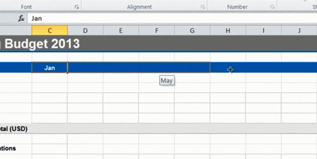
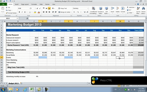
Here I have a simple template for a marketing budget for 2013 that I need to fill out. My template doesn’t have the months, so I’ll write “Jan” in the first cell and then I’ll position my mouse pointer in the bottom right corner of the cell and drag the fill handle to automatically fill the rest of the months.

Excel recognizes time series like months, days and quarters.

Now I’ll add the first budget item which is “Outsourced market research”. We pay a firm to do this for a fixed cost of 500 dollars a month. I’ll write 500 in the first cell and then I’ll grab the fill handle again to copy the number to all cells.

Using a formula to apply a 20% increase (01:50)

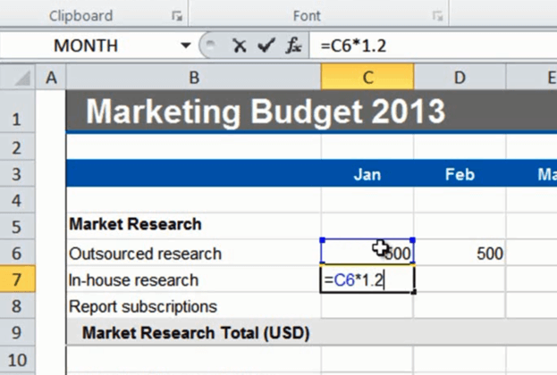
The next item, the “In-house research” is 20 percent more expensive than the outsourced market research so I’ll create a formula to calculate that number. I’ll mark the cell and write an equal sign, this is the way you start all formulas in Excel, then I’ll mark the “Outsourced research” number and multiply it with 1.2 to get the 20 percent increase and hit “Enter” to see the result.

There, that looks fine, so now I’ll grab the fill handle again and drag it across all columns to copy the formula. If I double-click one of the cells I can see that the formula takes the value above and multiplies it with 1.2. This is a so called relative reference, meaning that the formula is updated to reflect its location in the spreadsheet.

Filling multiple cells at once with the same value (02:43)

Next I want to fill out the “Report subscription” row. Again this is a fixed cost of 250 dollars each month. Instead of entering the number in the first cell and using autofill, I can mark all the cells where I want the value, write the number 250 and press “CTRL” +” Enter”. As you see, all the cells that I marked were filled at once.

Using “AutoSum” to calculate totals (03:09)

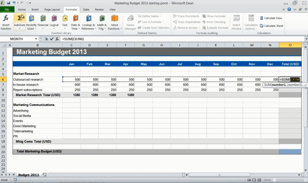
Now I want to add totals for this section. I’ll mark the cell where I want the total and click on the “AutoSum” icon with the Greek symbol Sigma ().

You can find it on the “Home” tab, or on the “Formulas” tab.

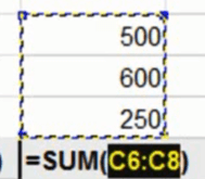
It will select the numbers in the range above and enter the formula =SUM(C6:C8).

Again I’ll press “Enter” to see the result. Now I can copy the formula by just dragging the fill handle to the right. You can do the same thing for the rows. Here I’ll position the marker in the first row total and click “AutoSum”.

But if I have numbers like this where I want to add up both the columns and the rows I can mark the entire range, including the empty cells where I want the totals to end up, and just click “AutoSum”.

This gives me all the totals I need in a split second.

Using formulas with fixed, “absolute” references (04:09)

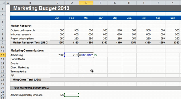
In the next section the first line item is “Advertising”. I’m not really sure how much to spend each month but I want to budget approximately 30,000 dollars on an annual basis and I want to incrementally increase the advertising with a certain percentage each month. I’ll start with 2000 in January. Now I want to test some different percentages so under my budget I’ll write, “Advertising monthly increase” and just start out with a percentage, let’s try 5%. I’ll enter a formula which says, take the value of the previous month plus an increase of 5% of that value. (=C12+C12*C22)

The result is 2100 dollars. Now, if I copy this formula to the right you’ll see that there is no change to the number. If I double-click the formula I can see that the formula is using the value in the cells one step to the right, so it’s not picking up the 5 percent increase.

I need to make sure that this cell, with the percentage, stays fixed.

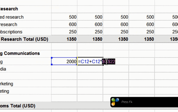
To do that I will go back to the original formula and create a so called “absolute” reference by adding a dollar sign before the column letter and the row number. The easiest way to do that is to go to the cell reference in the formula and press “F4” on your keyboard.

There, now I can apply that formula to the entire row. I’ll click “AutoSum” to see the total for the year. As you can see the total is more than 30,000 but now I can easily just change the percentage to say 4 percent.

The total is now slightly higher than 30,000, but that’s ok, I’ll leave it like that.

Changing the number format (05:59)

Now I got a lot of decimals that I don’t need. First I’ll change the number format to currency, to do that I’ll just mark all the cells where I have numbers, go to the “Home” tab and in the “Number” section I’ll select “Currency”.

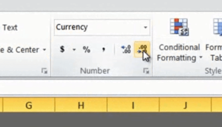
I’ll leave the default which is US dollars. Then I’ll reduce the number of decimals by clicking “Decrease Decimal” in the “Number” section.

This doesn’t delete the decimals it just hides them.

Removing formulas and keeping the values (06:27)

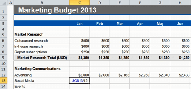
Next is “Social Media”. I want to spend 15,000 dollars on an annual basis distributed evenly throughout the year. So I’ll enter 15,000 in the total cell and then in the cell for January I’ll write the formula, an equal sign, and then the cell with the total and again I want to make this absolute so I’ll click F4, then I want to divide the total with 12 for the 12 months =$O$13/12

If I hold down “CTRL” when I click “Enter” I’ll stay in the current cell. Now I’ll apply this formula to the rest of the months. Perfect, I get 1250 dollars each month. But Now I need to change the formula of the total cell because otherwise if I later on manually change the value of a cell the total won’t update. To remove the formulas and only keep the values of these cells I’ll mark the numbers, right click, drag a little back and forth and then select to “Copy here as values only”.

If I double click you can see that the formula is gone, and we only have the value in the cell. Now I’ll just click “AutoSum” and now, as you can see, if I make changes here in a cell a new total is calculated. But I’ll just click “Undo” here for now.

Selecting and filling random cells with a value (07:50)

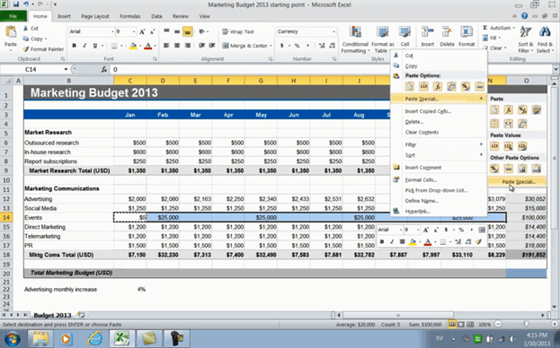
On the next row we have “Events”. We plan to have our events quarterly so I’ll mark the cell for the first event in February and then I’ll hold down “CTRL” and mark the cells for each quarter.

Now I’ll release “CTRL” and enter the amount 25,000 dollars and then I’ll hold down “CTRL” again and press “Enter”.

For the next line items, “Direct Marketing” and “Telemarketing” I’ll just add fixed monthly fees. I’ll mark the range, enter the amount 1,200 and then press “CTRL” + “Enter”. I’ll do the same for “PR”, mark the cell range write 1500 and then “CTRL” + “Enter”. To get the totals I’ll do like before, I’ll mark the cells including the total row and column and click “AutoSum”. There, now I have those totals!

Adding a “0” to empty cells (08:44)

Finally I’d like to fill the empty cells here with a zero, so to do that I’ll show you a little trick.

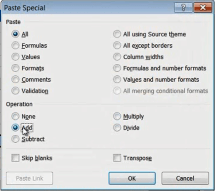
I’ll type “0” in one of the empty cells, copy it, mark the range that has empty cells, right-click, and select “Paste Special”.

Here, under “Operation” I’ll click “Add” and then “OK”.

There, now zero has been added to all cells.

Now for the final row. Here I’ll enter a formula to say “=”and then I’ll select the first subtotal for “Market research” and then “+” the second subtotal for “Marketing Communications”.

Now I can just drag that formula to the end to see my final total.

Closing (09:33)

If you know how to use simple formulas like the ones I showed you in this video, you’ll be able to add numbers to your spreadsheet that make sense to your business. If you also learn a few of the keyboard shortcuts you’ll be able to finish even faster. I’m Ulrika Hedlund for Business Productivity – thanks for watching!