
Sort and filter data to find answers
Introduction (00:04)
Quite often you have a spreadsheet with data that you need to make sense of. In this video you’ll learn how to sort and filter data to find answers to specific questions. You’ll learn how to sort data on multiple columns, how to sort on color and how to filter data based on different data types. Let me show you!
Checking for empty rows or columns (00:26)
Here I have a spreadsheet with data exported from our customer relationship system. Each row represents a sales opportunity. To sort data you first need to make sure that you have no gaps in your datasheet – that is, no empty columns or empty rows.
If you do have gaps, like I do here and you sort your data, Excel will only sort the data up to that gap and you will be left with inconsistent data.
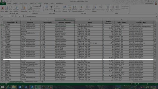
One way to check your data for empty columns or rows is to go to the end of the data range. To go the end of the data range horizontally, double click the right side of any cell in a row, or press the keyboard shortcut CTRL Arrow Right. Here I seem to have an empty column, but to make absolutely sure there is no data further down in the column I’ll press CTRL Arrow Down. Since this takes me to the very last cell of the spreadsheet I can be sure that this column is empty. I’ll press CTRL Arrow Up and then I’ll right-click and delete the column. To check for empty rows follow the same procedure downwards.
Sorting data by a single column (01:39)
Now I’d like to know how large our biggest deals are in terms of revenue. To sort your data, mark any cell in the column you want to sort by, here I’ll mark a cell in the “Product revenue” column. Click the “DATA” tab and in the “Sort & Filter” section select how you want to sort your data. In this case I want to see the largest numbers at the top so I’ll select the sort button named “ZA” which sorts largest to smallest.
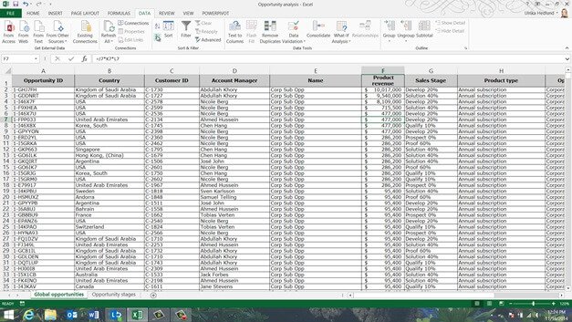
Immediately, I can see the largest numbers at the top. Now I get a much better understanding of this opportunity pipeline.
Sorting multiple columns after one another (02:16)
Now I’d like to know how many opportunities each account manager has and what type of opportunities these are, so I want to sort by two columns. To sort data by multiple columns, on the “DATA” tab, in the “Sort & Filter” section click the “Sort” button. Here you get the option to add multiple levels. First remove any previous sorting criteria by clicking “Delete Level” and then click “Add Level”.
In the “Sort by” drop down select the first column you want to sort by, I’ll select the “Account Manager” column. Then select what you want to sort and in what order. I’ll keep the default which is “Values” and “A to Z”. To add another sorting level click “Add Level” and select the second column. Here I’ll select “Opportunity Type”. Again I’ll leave the default, “Values” and “A to Z”. To apply the filter click “OK”.
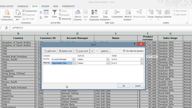
And now the data is sorted by these two columns. Here I can see that our account manager Abdullah has three consulting opportunities and the rest subscription opportunities.
Sorting in an order you define yourself (03:27)
Now I’d like to sort the data by “Sales Stage” to understand how many opportunities we are about to close. The “Sales Stage” column can contain one of the following values. I can’t sort this column alphabetically, because then I’ll get them in the wrong order, so I’ll have to sort them in a custom order that I define myself.
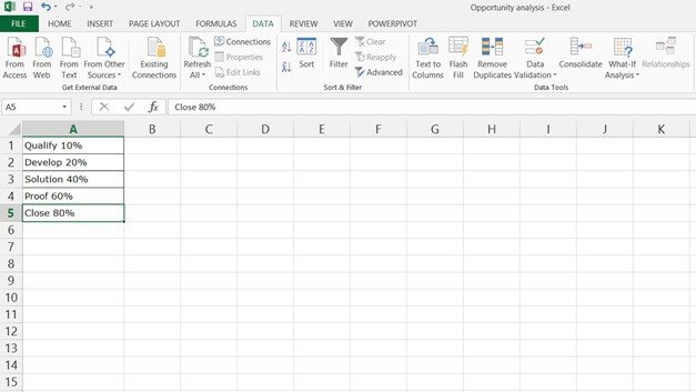
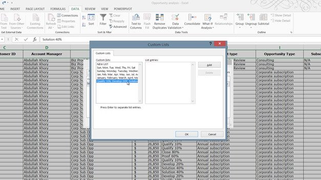
To sort data in a custom order, click the “Sort” button. Here I’ll delete any previous columns I’ve sorted by. Click “Add Level” and select the column you want to sort by. Here I’ll select the “Sales Stage” column. In the “Order” drop down select “Custom List”. Here Excel has a number of custom lists built in, so for instance you can sort data by day of the week or month of the year and so on. Here I’ll select “NEW LIST” and click “Add”. Now I can add my sales stages by typing them in and Excel will use this as the sorting order.
Another quicker way to do this is to click the “FILE” tab and then “Options”. Click “Advanced” and scroll all the way down until you see “Edit Custom Lists”.

Click the selection button and mark the list with your defined sort order and then click “Import”. As you can see, the list has now been added to the custom list of Excel.

Click “OK”, and then “OK” to close down the “Options” window. Click the “Sort” dialog box again and click “Add Level”. Select the column you want to sort by. In the “Order” drop down select “Custom List”, and as you can see, the list that you just imported is now available as an option.
Select it and click “OK”. Now you can see that the data has been sorted by “Sales Stage”.
Sort data by formatting such as color (05:20)
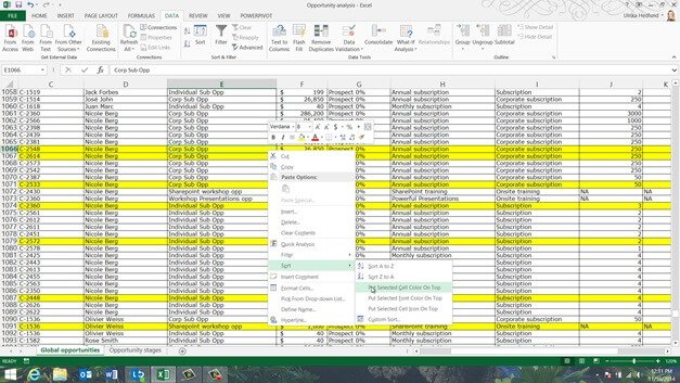
In addition to sorting on the values of cells, sometimes you want to sort by formatting, such as the color. Here you can see that I have a number of rows that have been highlighted with a different cell color. To sort data by formatting, mark a cell with the formatting applied, right-click and select “Sort”, Here I’ll select “Put Selected Cell Color on Top” since I want to sort on the cell color.
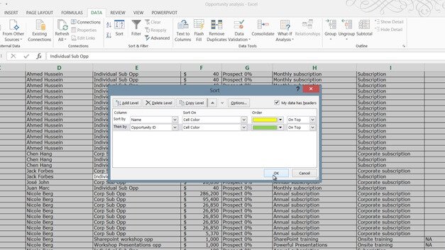
All yellow rows are now sorted on top. If you don’t want to scroll to find all colors, on the “DATA” tab, click the “Sort” button. Click “Add Level” here you can select any column since they are all colored, in the “Sort On” drop down select “Cell Color”. In the “Order” drop down you can see all the colors that are present in your spreadsheet. Here I’ll add the green color and click “OK”.
Now I have all the opportunities that have been highlighted in yellow at the top followed by the opportunities in green. I can quickly see that the ones that have been highlighted in green have been closed in just about ten days, whereas the ones that have been highlighted in yellow are still on the Prospect stage, even though they’re over 150 days old.
Sorting randomly (06:38)
Sometimes you want to sort data randomly. Say for instance that you randomly want to pick 10 opportunities to follow up on. To randomly sort your data you can use a function that Excel provides to generate random numbers. Mark the first data cell in the column next to your data range, write equal mark and then the function “RAND()”.
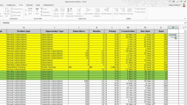
A random number between zero and one is automatically generated. Double-click the bottom right cell corner to generate numbers for all rows. To sort by this column, mark any cell in the column and on the “DATA” tab click sort “A to Z”. As you can see, the data has now been sorted completely randomly. Now you can right click and delete this column.
Filtering your data (07:27)
In addition to sorting, you can find answers by using filters. To filter your data mark any cell in your data range, on the “DATA” tab, in the “Sort & Filter” section click the “Filter” button. As you can see you get a little arrow next to each column name. Click on the arrow to see the various filter options. You can resize the filter window by just pulling the handle. Here you can deselect all values by un-checking “Select All” and then select what you want to filter on and click “OK”.
To clear the filter again click “Clear” on the “DATA” tab or click the column filter and select “Clear Filter from” the Column name.

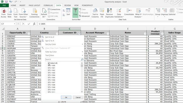
Depending on the type of data in the column, Excel provides you with different filers. Since this is a text field I get “Text Filters”. The “Text Filters” enable you to filter on fields containing specific characters. In Excel 2010 Microsoft introduced a new powerful search filter. Say for instance that I want to see all opportunities from the customers with customer ID 1610 and 2398. I’ll type in 1610 in the search field and click “OK” to see all opportunities related to that customer ID.

I’ll click “Filter” again and write in 2398. To keep the initial results I’ll mark the option to “Add current selection to filter”. Now if I click “OK”, I get both customer IDs. If I go to the “Product revenue” filter, you can see that I here have “Number Filters”. Here I want to find our top 10 deals so I’ll click Top 10 items and click “OK”.
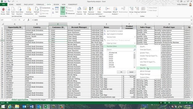
Now I can see the top ten opportunities based on “Product revenue”.
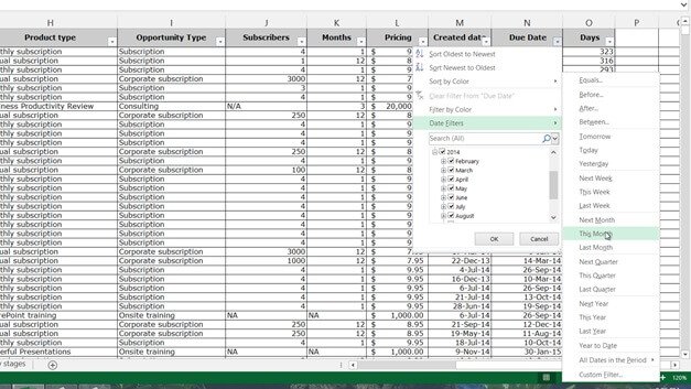
Finally let’s have a look at a date filter. Here I’ll filter the “Due date” column. As you can see the filter options are neatly organized in years and months. Excel provides me with a number of “Date Filters”. Here I’ll filter “This Month” to see only the opportunities that are due this month.
Closing (09:46)
Now that you know how to effectively sort and filter data, you’ll easily be able to find answers hidden in large data sets.