How to hide columns and rows
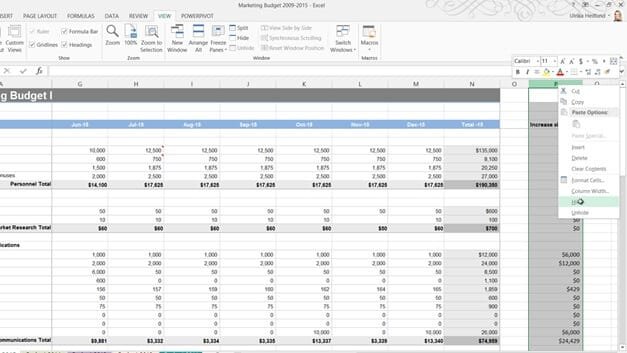
To hide a column, right-click and select “Hide”.
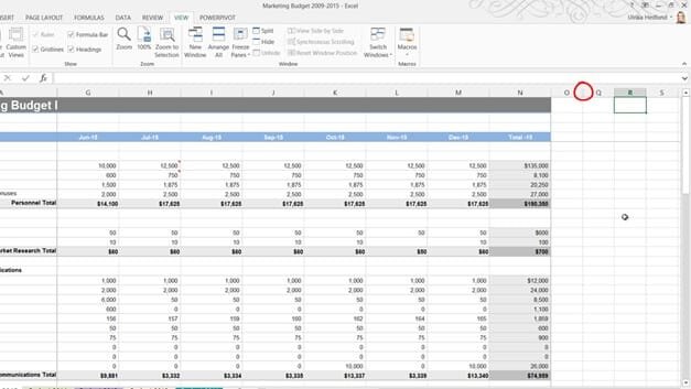
You can see that the column is hidden because there is a gap between O and Q. In Excel 2013 hidden columns and rows are easier to spot since they are also shown with a double line.
Now I only want to show the last quarter so I’ll mark the nine first months, right-click and “Hide”. To mark multiple, un-adjacent rows or columns hold down the CTRL key on your keyboard. Here I’ll mark all the budget item rows where we haven’t allocated any money in the budget. I’ll release the CTRL key, right-click and select “Hide”.
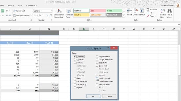
To get a better overview of all hidden rows and columns, on the “HOME” tab, click “Find & Select”, “Go To Special” and select “Visible cells only” and click “OK”.
As you can see all hidden rows and columns are marked with white lines, making them easier to see.


