How to filter data in Excel 2010
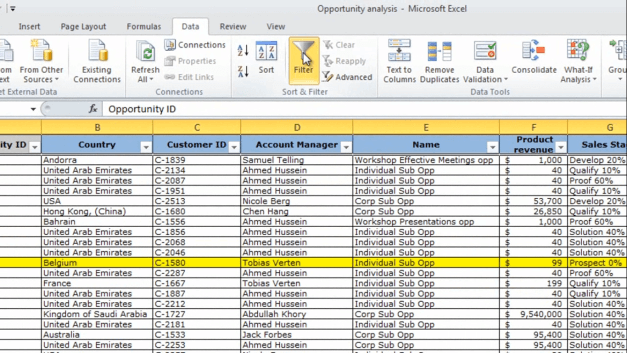
To add filters to your data just mark the first row with your headers and click the Filter button.
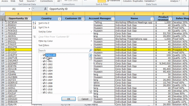
As you can see you get a little arrow next to each column name and here you get the filter options. You can resize the filter box by just pulling the handle. I can deselect all by clicking Select All.
And then I can select the values I want to filter on. Excel also recognized different types of data in your column and gives you different filters. Since this is a text field I get Text Filters.
So for instance I can select “Contains” Customer-ID with the number “1610”, or containing “2398” and click “OK”,
and here you can see all the opportunities related to those customers. To clear the filter I’ll just click “Clear”.
Another very powerful way to filter is by using the search field. So here I can just type “1610” and click “Enter” and again I get all of the opportunities related to that customer.
If I go to the product revenue filter, you can see that I here have “Number Filters.” I’ll click “Top 10”.
But instead of “Items”, I’ll select “Percent” and click OK. And here they are: my top 10% deals.
Finally let’s have a look at a date filter, so if I look at the due date for these opportunities I get date filters from excel. So here I can easily filter on different date fields.


