How to create a pivot table in Excel 2010?
To create a PivotTable, click any cell in the table, click “Insert” and then click “PivotTable”.
Excel selects the table range for you and you can select where you want the PivotTable to be placed. I’ll just leave the default, which is in a New Worksheet and then click OK.
There, now I have my PivotTable on the left and my field list on the right.
You use the field list to select which data you want to see in your PivotTable.
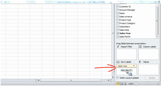
Now the first thing I’d to look at is total sales per month for 2011 and 2012. So to create that PivotTable I’ll first select “Sales Year” and drag it to the Row Labels area. Then I’ll select “Sales Month” and put it under “Sales Year”.
And then I’ll take the “Sales revenue” that I want to be added and put it in the Values section, and there is my PivotTable!


