How to create a PivotTable
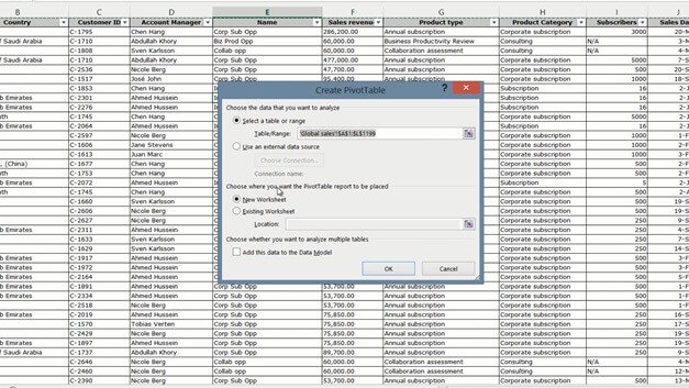
To create a PivotTable start with a data set with at least one column of numerical information that can be totaled or compared. Here I have sales transactions for 2013 and 2014. Click any cell in your data range, click “INSERT” and then click “PivotTable”. Excel selects the data range for you and you can select where you want the PivotTable to be placed. I’ll just leave the default, which is to insert it into a New Worksheet and then click OK.
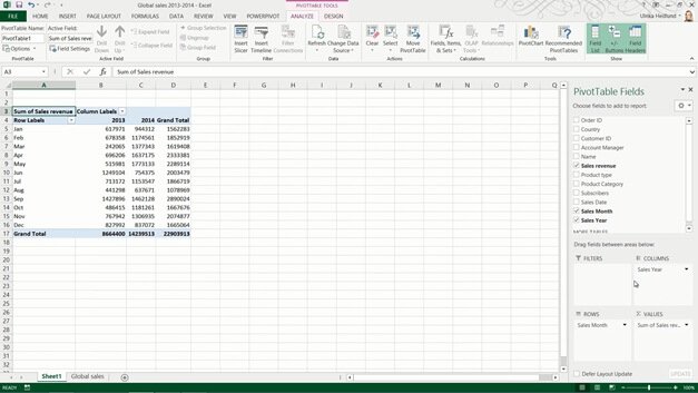
To analyze data in a PivotTable you need to add number fields to the Values area. I’ll select the Sales Revenue field. Right away you can see the total sum of sales revenue for 2013 and 2014 combined.
Now you can move data fields to the row and column areas to see the breakdown by year, by month and by any other column that you had in your data range. You can switch between various views and filters to analyze your data from various perspectives.


