Automate calculations with LookUps
Introduction (00:04)
Sometimes when you are doing calculations you need to base your numbers on a certain criteria. For example, the amount you pay your employees might depend on how well they have performed. In this video you will learn how to use lookup functions in Excel to fine-tune your calculations.
Showing formulas in a spreadsheet (00:23)
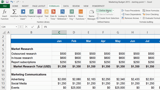
Here I have a marketing budget that I’ve started to fill out.
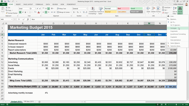
Some of these numbers I’ve added manually, but some of them are calculated using formulas. To get a good overview of all the formulas in a spreadsheet you can go to the “Formulas” tab and in the “Formula Auditing” section click “Show Formulas”.
Now all the formulas in the spreadsheet become visible. You can also access this by pressing the keyboard shortcut CTRL + Accent Grave or CTRL + Tilde if you have a US keyboard. To go back to the normal view again I’ll click “Show Formulas”. Another way to get a good overview of the formulas in your spreadsheet is by highlighting those cells. You can do that by going to the “Home” tab, and in the “Editing” section click “Find & Select” and then in the drop down select “Formulas”.
All the cells with formulas will be selected. If you want to have better visibility of these cells you can highlight them using a different cell background color. I’ll click “Undo” here to go back to the original cell color.
Using the “IF” function (01:34)
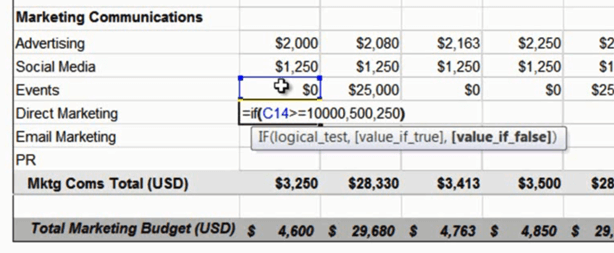
Now I’m going to continue filling out this budget, so I’ll go to the first empty line item which is “Direct Marketing”. Here I want to allocate a fixed monthly amount of 250 dollars but the months where we are investing a lot of money on events, 10,000 dollars or more, I want us to double that amount and make it 500 dollars. Instead of manually tracking which months have 10,000 dollars or more budgeted for events I’m going to use a lookup formula which will do this for me. I’ll start by entering an equal sign to start the formula, then I will write IF, left parenthesis and here I can see that Excel helps me with the formula.
First I have to enter the so called “logical test”, so I’ll say, if the budgeted cost for the event that I have for January in cell C14 is larger (>) or equal (=) to 10,000, and then a comma, then the direct marketing budget should be 500 so I’ll type 500 and then a comma again, otherwise it should be 250. I’ll complete the formula with a right parenthesis.
There! Now, let’s copy this formula to all the cells to see if we get the right result. That looks right. The months where we have the events that cost ten thousand or more we spend 500 dollars in direct marketing, otherwise we spend 250.
Using formulas in your IF statement (03:09)
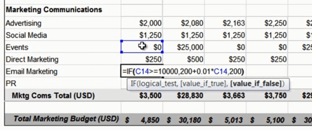
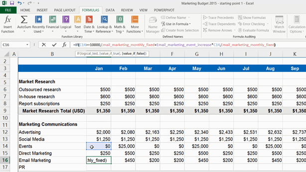
For email marketing we have a fixed monthly fee of 200 dollars, but the months where we have events that cost 10,000 or more I want to add an additional 1 percent of the event cost to the 200 dollars. So to do that I need to add some more calculations to my IF statement.
I’ll start with an equal sign, type IF again and left parenthesis, for the logical test I’ll first mark the cell containing the Events cost for January; C14, if this is larger (>) or equal (=) to 10,000 dollars, comma, if this is true I’ll add 200 dollars, plus (+) 1 percent times (*) the event cost, comma, otherwise I’ll just add 200 dollars. I’ll end with a right parenthesis and then “Enter”.
Now, I’ll copy this formula again across all the months. You can see that I now have more money allocated for email marketing each quarter when I have my large events.
Make your formulas easier to read with named cells (04:10)
If you use a value over and over again, or if you want to test different scenarios by changing values, or if you just want to make your formulas easier to read, you can give your cells a name. Let’s change the email marketing formula and make use of named cells instead.
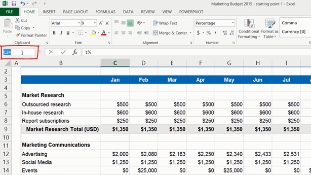
First I’ll type “Email Marketing monthly fixed” and enter the 200 dollars which is the fixed cost every month in the cell to the right. Then I’ll write “Email Marketing event increase” and enter the 1%.
Instead of referring to these cells as C23 and C24 I will name them. There are multiple ways in which you can name your cells. You can mark the cell and type in a name in the text box up here,
I’ll click ESC to show you another way.
If you go to the “Formulas” tab and click “Define Name” you can enter the name here in this text box. Excel has automatically taken the text to the left of the cell and added it as a name with underscore signs instead of spaces. You can keep this name or change it here in the textbox.
I’ll click Cancel and show you the third way. Mark your cells, the ones with the names and the ones with the values and click “Create from Selection.”
Here you need to tell Excel which cells you want to use for the name, and in our case its’ the cells to the left, and then Excel creates the names for me. If you click “Name Manager” you can see all the names you have in your spreadsheet. Here you can add new names, or change and delete existing names in your spreadsheet.
Use cell names instead of numbers (06:08)
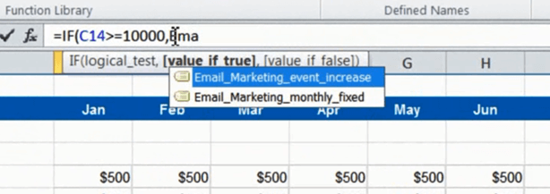
So let’s go back to our formula again and use these cell names instead of numbers. As I start typing the name you will see all the matching names appear in the drop down box.
Here I want to select the fixed fee which is the bottom one so I’ll press arrow down on my keyboard and then press TAB to select the highlighted option. Then I’ll add the percentage increase and multiplied with the amount budgeted for the event. I’ll add a comma and then enter the name for the fixed fee. I’ll end with a right parenthesis and press Enter.
Now I’ll copy this updated formula across all months.
Now I can easily try different scenarios. Say for instance that I want to increase the fixed amount to 250 dollars and the percentage increase to 3%. I can see the results in my budget right away.
Using the VLOOKUP formula to look up values (07:05)
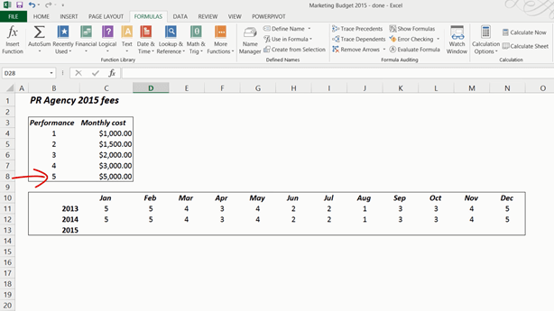
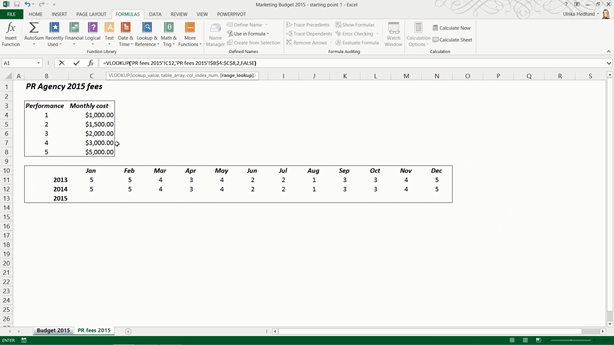
Next I want to budget for our PR. Our PR agency charges different fees depending on their media outreach performance. If their performance is 5, the cost is 5000 dollars a month, if it’s 4 it’s 3000 and so on.
For budgeting purposes I’ll just assume that they will have the same performance this year as last. Now I need a formula that can check the performance number for the month, look it up in this table and give the value in this column.
I’ll go to my budget and enter the formula: Equal sign (=) and then I’ll start typing VLOOKUP and select it in the drop down list by pressing TAB on the keyboard. First is the “lookup_value”, this is the value I want to look up in the table, so I’ll go back to my PR sheet and mark the first cell for January and then I’ll press comma, to enter the “table_array”, here I need to mark the columns in my lookup table with values, I won’t include the headers,
here I’ll press F4 to make the table absolute, meaning that if I copy the formula it should always refer back to these exact cells for the lookup table.
I’ll press comma again to get to the next value which is “column_index_number”, this is the number of the column of your lookup table that has the value that should be returned, in our case it’s the 2nd column that contains the values. Finally I’ll press comma again and here I can select TRUE or FALSE. False means that the numbers are exact, meaning that there is no performance of 4.5.
OK, let’s try this. The first result is 5000 which is correct, now I’ll just copy the formula across all months. There! It worked! Now we are done fine-tuning our budget!


